Modeling with satellite observations

Model a mesoscale eddy with WaveVortexModel and compare how current altimetry missions sample it.

Source: Examples/Tutorials/Modeling.m

Initialize the model domain

We start with a barotropic quasi-geostrophic domain large enough to watch one mesoscale eddy translate across the basin while the active missions sample it along their native ground tracks.

Lx = 2000e3;
Ly = 1000e3;
Nx = 2*256;
Ny = 2*128;
latitude = 24;

wvt = WVTransformBarotropicQG([Lx, Ly], [Nx, Ny], h=0.8, latitude=latitude);

Add a Gaussian eddy

The initial sea-surface height anomaly is

\[\eta(x,y)=A\exp\left(-\frac{(x-x_0)^2 + (y-y_0)^2}{L^2}\right),\]

so the tutorial begins from one isolated anticyclonic feature.

x0 = 3*Lx/4;
y0 = Ly/2;
A = 0.15;
L = 80e3;
wvt.setSSH(@(x, y) A*exp(-((x-x0).^2 + (y-y0).^2)/L^2), shouldRemoveMeanPressure=true);

figure(Position=[100 100 760 320])
pcolor(wvt.x/1e3, wvt.y/1e3, 100*(wvt.ssh).'), shading interp
axis equal tight
xlabel("x (km)")
ylabel("y (km)")
title("Initial sea-surface height anomaly")
colorbar

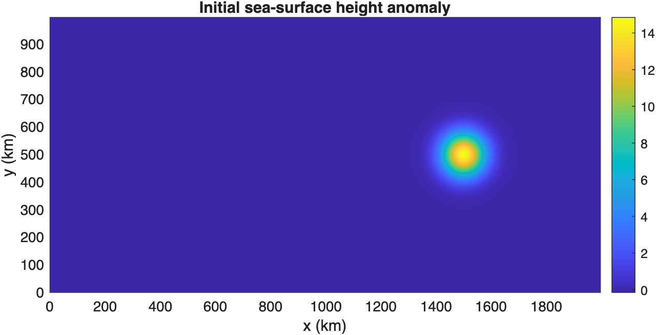
The Gaussian eddy starts as one compact sea-surface height anomaly centered away from the boundaries.

Add the background dynamics

We add adaptive damping and beta-plane advection before launching the model integration.

wvt.addForcing(WVAdaptiveDamping(wvt));
wvt.addForcing(WVBetaPlanePVAdvection(wvt));
model = WVModel(wvt);

Add the active altimetry missions

The along-track output group samples the model with the geometry of each currently operating mission.

netcdfPath = string(tempname) + ".nc";
cleanupNetCDF = onCleanup(@() deleteTemporaryFile(netcdfPath)); %#ok<NASGU>
outputFile = model.createNetCDFFileForModelOutput(netcdfPath, outputInterval=86400, shouldOverwriteExisting=true);
model.addNetCDFOutputVariables("ssh", "zeta_z");

ats = AlongTrackSimulator();
currentMissions = ats.currentMissions;
for iMission = 1:length(currentMissions)
    outputFile.addOutputGroup(WVModelOutputGroupAlongTrack(model, currentMissions(iMission), ats));
end

Integrate for one year

This gives the eddy time to translate westward while the repeat and drifting missions build up different spatial sampling patterns.

model.integrateToTime(365*86400);
outputFile.closeNetCDFFile();

figure(Position=[100 100 760 320])
pcolor(wvt.x/1e3, wvt.y/1e3, 100*(wvt.ssh).'), shading interp
axis equal tight
xlabel("x (km)")
ylabel("y (km)")
title("Sea-surface height after one year")
colorbar

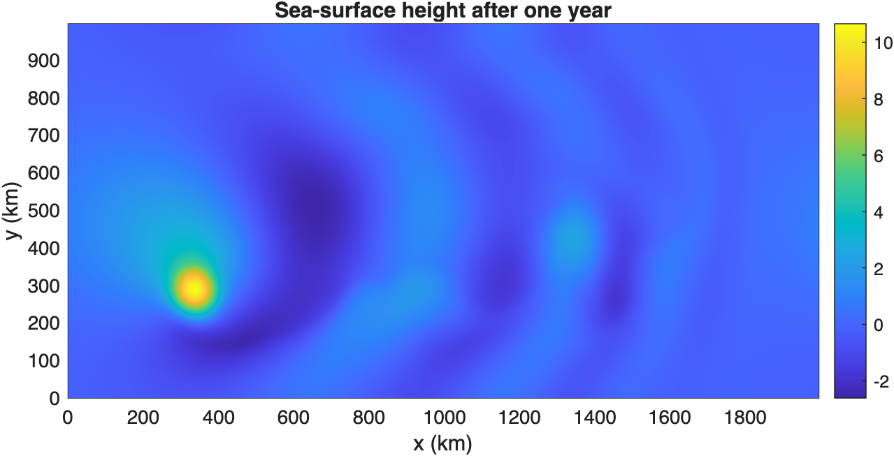
After one year the eddy has propagated westward and broadened under the model dynamics.

Render the satellite sampling movie

The movie combines the full field with three observation views: the reference mission, the reference-plus-interleaved pair, and all active missions together.

movieSettings = modelingMovieSettings(currentMissions);

Daily snapshots of the full field are shown with the reference mission, the reference-plus-interleaved pair, and all active missions using a four-day fading window around each frame.

The upper-left panel shows the full model field.

The upper-right panel shows the reference mission, Sentinel-6A, with a four-day fade before and after each frame so the repeat-track pattern is visible.

The lower-left panel adds the interleaved Jason-3 orbit to show how the staggered pair fills gaps between successive Sentinel-6A passes.

The lower-right panel overlays all active missions to show how the full constellation samples the eddy.