Modeling with satellite observations
This tutorial uses the WaveVortexModel to model the evolution of a mesoscale eddy. The AlongTrackSimulator samples the sea-surface of the model in the sampling pattern of the current altimetry missions.
Model initialization
Set up the model domain
Lx = 2000e3;
Ly = 1000e3;

Nx = 2*256;
Ny = 2*128;

latitude = 24;

wvt = WVTransformBarotropicQG([Lx, Ly], [Nx, Ny], h=0.8, latitude=latitude);
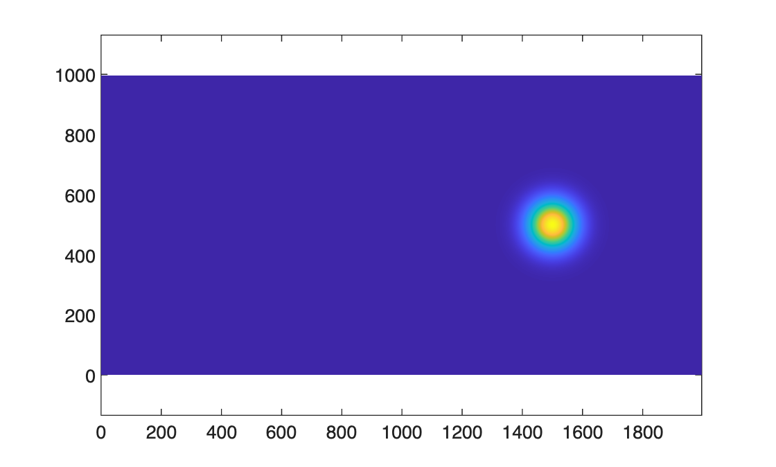
Add a gaussian eddy
x0 = 3*Lx/4;
y0 = Ly/2;
A = 0.15;
L = 80e3;
wvt.setSSH(@(x,y) A*exp( - ((x-x0).^2 + (y-y0).^2)/L^2),shouldRemoveMeanPressure=1 );

figure, pcolor(wvt.x/1e3,wvt.y/1e3,wvt.ssh.'), shading interp, axis equal
Add small scale damping, beta-plane advection, and initialize the model
wvt.addForcing(WVAdaptiveDamping(wvt));
wvt.addForcing(WVBetaPlanePVAdvection(wvt));
model = WVModel(wvt);
Use the simulator to add all current altimetry missions
outputFile = model.createNetCDFFileForModelOutput('QGMonopoleWithAlongTrack.nc',outputInterval=86400,shouldOverwriteExisting=1);
model.addNetCDFOutputVariables("ssh","zeta_z")
ats = AlongTrackSimulator();
currentMissions = ats.currentMissions;
for iMission = 1:length(currentMissions)
    outputFile.addOutputGroup(WVModelOutputGroupAlongTrack(model,currentMissions(iMission),ats));
end
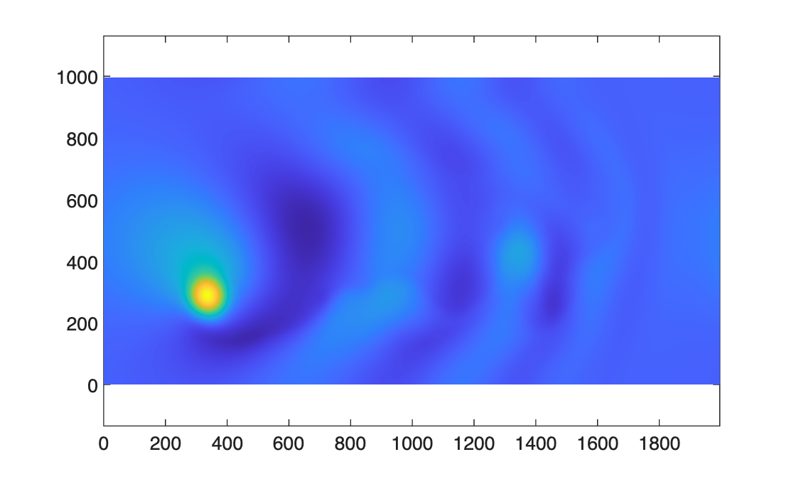
Run the model for one year
model.integrateToTime(365*86400);

figure, pcolor(wvt.x/1e3,wvt.y/1e3,wvt.ssh.'), shading interp, axis equal
Visualizing the satellite observations
Using the NetCDF output file, we can use a script to make a movie that shows the evolution of the eddy, and different combinations of satellite observations of that eddy.
- The panel in the upper-left shows daily snapshots the sea-surface of the entire domain as the eddy propagates westward.
- The upper-right panel shows how the reference mission, Sentinel 6a, samples the eddy. For visualization purposes, we fade in the observations 4 days prior, and fade out 4 days after. In practice, the satellite passes over in a few minutes.
- The lower-left panel shows the combined reference and interleaved missions. The interleaved mission is on the same orbital as the reference mission, just shifted so the tracks create a staggered grid.
- The lower-right panel shows all the current missions. These include satellites with other orbits, including geodetic and drifting orbits.